Kriging and uncertainty
Ordinary, Universal, Empirical Bayesian and Indicator kriging; spherical, exponential, Gaussian, Matérn and linear variograms; leave-one-out cross-validation and prediction variance.
Use GeoAgent for guided natural-language execution, the core server for dependable built-in functions, DuckDB for spatial SQL, Pyodide for browser-local Python and an optional Python service for native geospatial and machine-learning libraries.
Each execution path has a deliberate role and can return portable GeoJSON, rasters, tables, profiles or service registrations.
| Runtime | Best for | Representative capabilities | Deployment behavior |
|---|---|---|---|
| Core server functions | Low-dependency, concurrent server operations and edge deployment | Geometry, topology, terrain, routing, catalogs, service translation, streaming, mission workflows | Built into the same headless server binary; no Python dependency |
| DuckDB spatial | Fast analytical SQL over local, database and cloud-native data | Spatial joins, aggregation, CQL2 execution, dynamic MVT, GeoParquet/object-store query, H3 and time-series workflows | Embedded analytical engine with spatial/httpfs and optional cloud extensions |
| Pyodide / WebAssembly | Interactive browser analysis with zero server compute | Python console, GeoPandas/Shapely-style processing, data transforms and notebook cells that drive the map | Runs inside the browser sandbox; packages and memory are constrained by WebAssembly/browser support |
| Python capability service | Native Python packages, long-running jobs, ML and specialist geoprocessing | WhiteboxTools, rasterio, scikit-learn, gstools, pykrige, OR-Tools, spaCy, Py6S, MegaDetector, BirdNET, virtualizarr and document generation | Optional isolated service with 176 routes; the core server continues operating when it is absent |
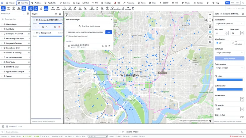
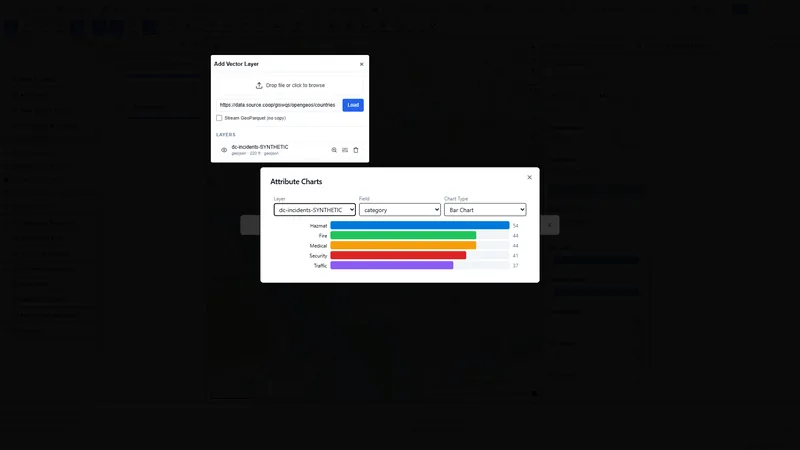
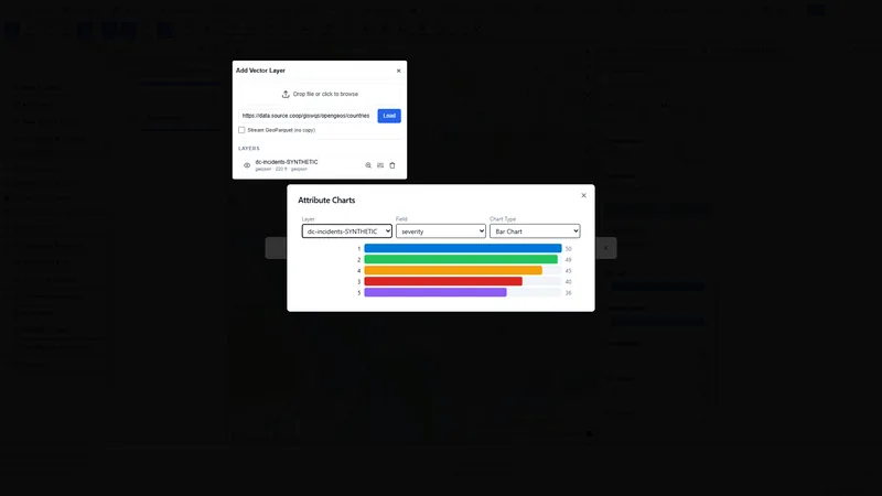
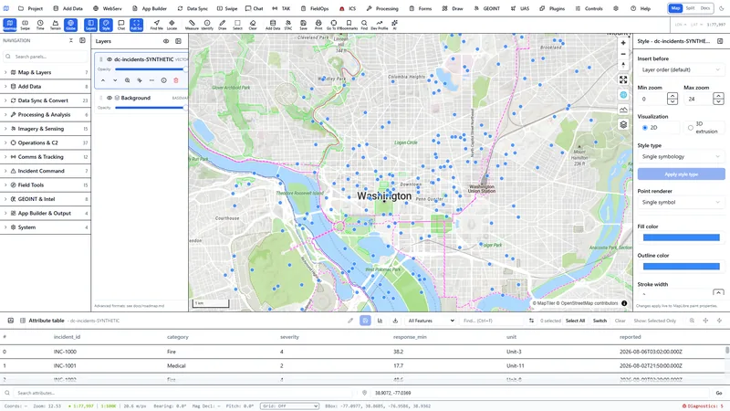
Data shown is a synthetic 220-point set generated for this capture, not real incident records. What it demonstrates is real: browser-side vector load and live DuckDB-WASM/Pyodide aggregation with no server round-trip per chart — the compute path documented in the table above, not the JupyterLite notebook UI described further down this page.
The same synthetic dataset shown above, loaded and charted against the real client — same synthetic-data caveat applies.
The analytics surface is intended to replace real operational workflows, not merely demonstrate buffers and centroids.
Ordinary, Universal, Empirical Bayesian and Indicator kriging; spherical, exponential, Gaussian, Matérn and linear variograms; leave-one-out cross-validation and prediction variance.
OLS with Moran’s I diagnostics, GWR/MGWR, LISA HH/LL/HL/LH clusters, Ripley functions, random forests with spatial cross-validation and space-time patterns.
D8 flow, depression fill/breach, stream extraction and ordering, watershed/sub-basin delineation, pour-point snapping, wetness index and upstream length.
Viewshed, skyline, slope, aspect, cut/fill, solar radiation, surface area, DEM draping, 3D buffers and terrain-aware routing.
Vehicle routing with constraints, origin-destination matrices, p-median/p-center, location set covering and maximal covering facility siting.
Raster function DAGs, band math, classification, convolution, atmospheric correction, change detection, segmentation, object detection and pixel-to-ground results.
Extract text from PDF, DOCX, PPTX and XLSX; run semantic search and citation-bearing RAG; identify 15 entity types, extract relations and push Cytoscape-compatible graphs into activity-based intelligence workflows.
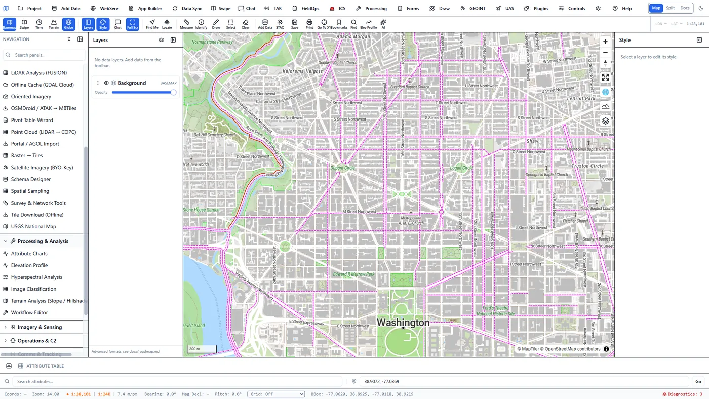
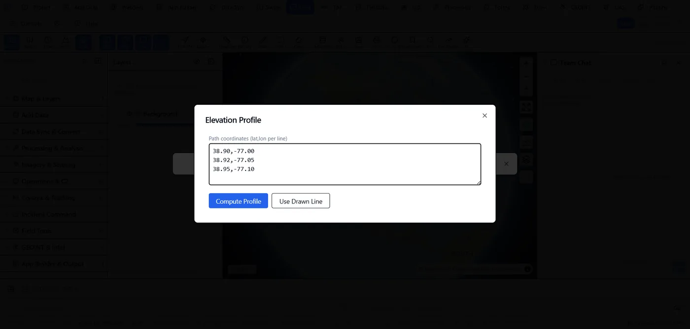
GeoAgent registers governed geospatial capabilities for imagery, kriging, routing, hydrology, statistics, topology, terrain and operations. It exposes the selected tool and parameters, then returns rendering hints for maps, rasters, profiles and tables.
Use the agent for guided execution and repeatable tool calls. Use notebooks for exploratory analysis, custom code, peer review, narrative and reproducible research. Both call the same underlying service and job APIs.
GeoLibre’s notebook work is not just a concept. The checked-in build and documentation define a dual-mode architecture with shared map scripting.
The web build stages a JupyterLite application inside the notebook panel and runs the Pyodide kernel entirely in the browser.
The desktop path launches a uv-managed JupyterLab server for native packages and a full Python environment.
Notebook cells can drive the live map and project state through the same scripting API used by the Python console.
The geolibre package is designed for local Jupyter, VS Code, Colab and JupyterHub-style environments with a leafmap-like API.
Runtime overrides allow Pyodide and DuckDB Spatial assets to be hosted locally for secure or disconnected environments.
Do not rebuild notebook UI or kernels from scratch. Keep JupyterLite for zero-infrastructure browser work, and add a governed multi-user server tier for workloads that need native packages, scheduled execution and enterprise controls.
A server-managed JupyterHub/Jupyter Server deployment integrated with 3DGeoServEngine identity, catalogs, service tokens, job scheduling and map/project APIs.
| Capability | JupyterLite / Pyodide workspace | 3DGeoServ Notebook Service |
|---|---|---|
| Compute location | User’s browser via WebAssembly | Containerized server kernels, optionally GPU-enabled |
| Native geospatial libraries | Only packages compatible with Pyodide/WASM | GDAL, rasterio, GeoPandas, PyTorch, WhiteboxTools and organization-specific environments |
| Large data | Limited by browser memory, sandbox and network behavior | Server-side access to databases, object storage, local high-speed storage and distributed services |
| Multi-user governance | Browser-local workspace | SSO/RBAC, per-user workspaces, quotas, image allowlists, audit events and network policy |
| Automation | Interactive, user-driven execution | Scheduled jobs, parameterized notebooks, headless execution, retries, logs and artifacts |
| Secrets | Avoid durable privileged credentials in browser code | Vault/Kubernetes secret injection, scoped service tokens and credential rotation |
| Deployment | Static, self-hosted JupyterLite assets | JupyterHub/Jupyter Server on Docker or Kubernetes, with air-gapped image registry support |
Start with integration and governance around mature Jupyter components, then add differentiating geospatial workflows.
Stabilize project/map synchronization, notebook file persistence, self-hosted runtime assets and repeatable example notebooks.
Deploy JupyterHub with curated CPU/GPU images, persistent volumes, SSO/RBAC and scoped 3DGeoServEngine tokens.
Schedule parameterized notebooks, capture logs/artifacts and publish outputs back as COG, FeatureServer, MVT, STAC or reports.
Add quotas, image promotion, package provenance, audit, cost controls, HA and disconnected deployment profiles.